Space Weather Lab

Learn — A university-level primer for radio amateurs

This guide explains what “space weather” numbers mean, why they change, and how they affect reception and propagation. It’s written for technically curious operators: you don’t need to be a physicist, but we won’t insult your intelligence.

Open the long-form University Primer

1) The ionosphere is your (variable) lens

Most long-haul HF communication relies on refraction in the ionosphere: a set of partially ionized layers produced mainly by solar radiation. Those layers are not static; they are a dynamic plasma whose electron density changes with solar illumination, season, latitude, and geomagnetic activity.

Two practical consequences:

Refraction limits: a path is supported only up to some maximum usable frequency (MUF).
Absorption limits: a path may be unusable at low frequencies due to D‑region absorption (raising the LUF).

Key ideas

MUF

Upper limit

Highest frequency likely to support a given path at a given time

LUF

Lower limit

Lowest frequency likely to work, mainly set by absorption and noise

2) What drives electron density (and why you care)

Electron density increases when the Sun deposits more EUV/X‑ray energy into the upper atmosphere. More ionization usually means better refraction for higher HF frequencies (think 20m/15m/10m opening more often), but solar activity can also create disruptive events (flares, CMEs) that make propagation worse.

A helpful mental model is to separate “slow-moving baseline” from “fast disturbances”:

Baseline (days to years): solar cycle, seasonal effects, day/night, latitude.
Disturbances (minutes to days): solar flares (R‑events), geomagnetic storms (G‑events), radiation storms (S‑events).

Visual examples (live SWPC products)

These images are published by NOAA/SWPC and update frequently. They’re useful for building intuition: you’ll start recognizing “HF absorption”, “solar wind turning south”, and “aurora likely” patterns at a glance.

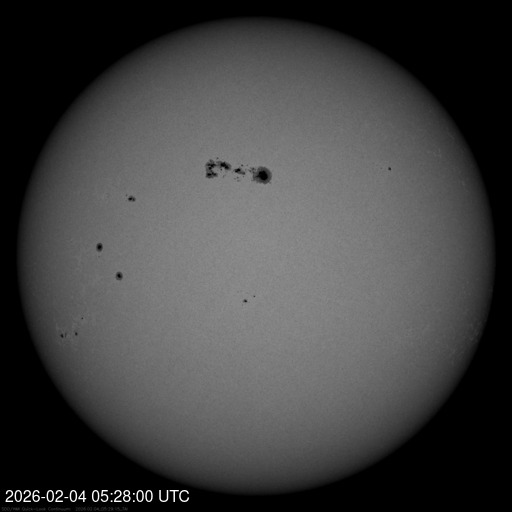
Solar disk (sunspots — white light)

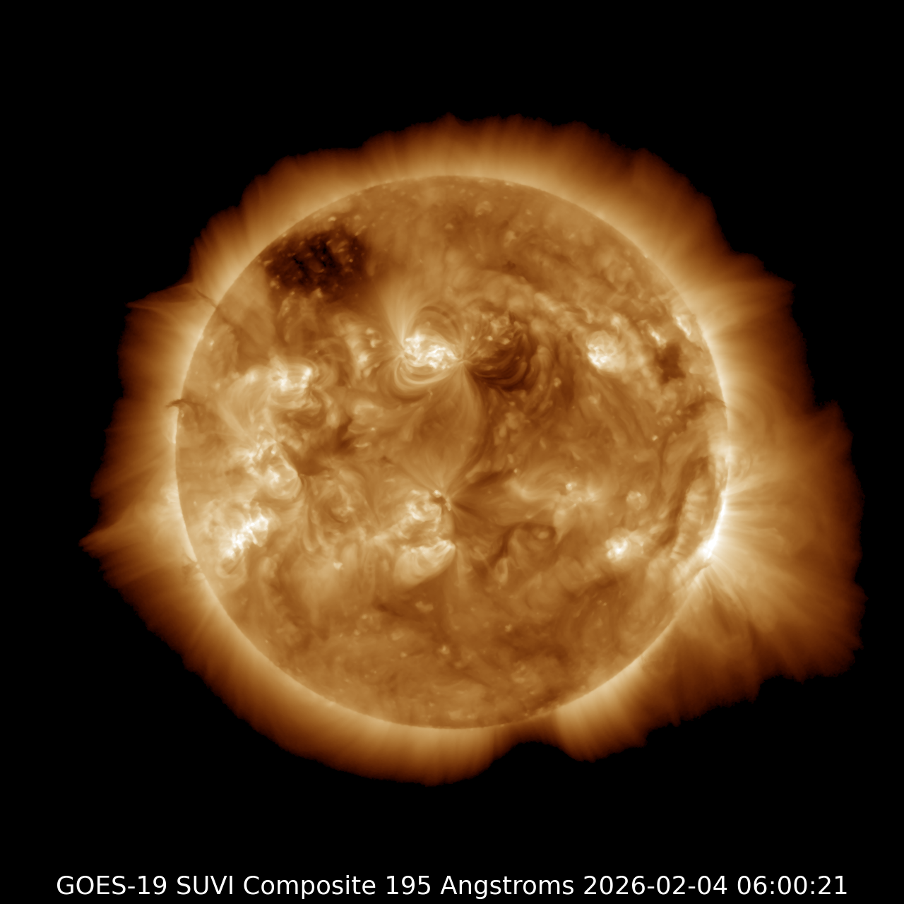
SDO/HMI intensity image showing sunspots — Sunspots are visible markers of strong magnetic fields. Regions with large/complex spots are more likely to produce flares, which can trigger sudden dayside HF absorption (R events).

Solar disk (active regions — color EUV 195Å)

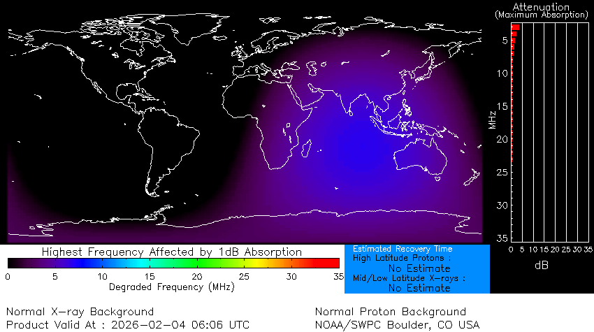
GOES-R SUVI 195 angstrom EUV image (false color) — EUV highlights hot coronal structures over active regions (false color). Bright/structured areas can be a visual “heads up” to watch X‑ray flux/R scale for flare-driven HF fadeouts.

D‑RAP (HF absorption)

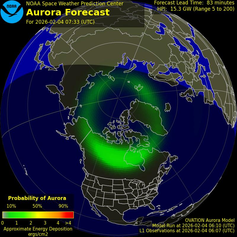
D-RAP global HF absorption map — When the dayside lights up, expect higher LUF and weaker HF—especially on lower bands.

Aurora forecast (Northern Hemisphere)

Solar wind + IMF (ACE MAG + SWEPAM)

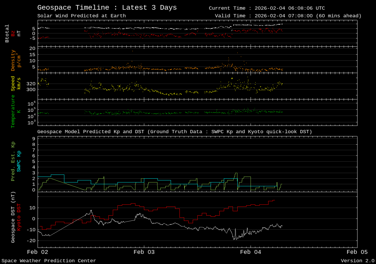
ACE magnetometer and solar wind (24 hour) — A sustained negative Bz (south) with faster wind is a classic recipe for geomagnetic activity.

Geospace (recent geomagnetic conditions)

Geospace geomagnetic activity plot (3 day) — Good for context: did a storm just happen, and is the system settling down?

3) F10.7 Solar Flux (SFI): what it is

The F10.7 index is a measurement of solar radio emission at 10.7 cm (2800 MHz). It is widely used as a proxy for solar EUV output. For HF ops, treat it as a “how ionizable is the ionosphere today?” baseline indicator.

Higher F10.7 generally supports higher MUF (more frequent 15m/10m openings).
F10.7 does not guarantee a band is open; it just improves the odds.
Local time and path geometry still dominate: a great day for Europe may be mediocre for the Pacific (and vice versa).

4) Kp and geomagnetic activity: what it means on-air

Kp is a planetary index describing geomagnetic disturbance. When Kp rises, HF paths—especially polar routes—often degrade. You may see increased fading, flutter, absorption, and shifts in workable frequencies.

Polar paths: tend to fail first as geomagnetic activity increases.
Lower bands: can sometimes remain usable when higher bands become unstable, but absorption and noise set the floor.
VHF+: geomagnetic storms can create auroral propagation (amazing, but geographically constrained).

5) NOAA R/S/G scales: operational severity summaries

NOAA summarizes space weather impacts using three practical scales:

R (Radio Blackouts): mainly driven by solar flares and X‑ray flux; affects HF absorption on the sunlit side.
S (Solar Radiation Storms): elevated energetic protons; can impact polar HF and satellites.
G (Geomagnetic Storms): geomagnetic activity; impacts HF/VHF propagation and aurora.

These are excellent “at-a-glance” numbers, but they intentionally compress a lot of physics. Use them as your alerting system, then drill into details.

6) Practical operating tips (informed by the physics)

High F10.7 + low Kp: try 15m/12m/10m; watch for openings near local noon and along grayline.
Low F10.7: expect 40m/80m to carry the long-distance load; daytime 80m may be absorption-limited.
R events (flares): if HF dies suddenly on the dayside, check the R scale; move to lower frequencies or different paths.
High Kp / G storms: avoid polar routes; try equatorial paths; consider NVIS if regional comms matter.
Always validate: propagation models are statistical; a quick WSPR/FT8 scan can confirm reality fast.